Single-cell transcriptomics yields ever growing data sets containing RNA expression levels for thousands of genes from up to millions of cells. Common data analysis pipelines include a dimensionality reduction step for visualising the data in two dimensions, most frequently performed using t-distributed stochastic neighbour embedding (t-SNE). It excels at revealing local structure in high-dimensional data, but naive applications often suffer from severe shortcomings, e.g. the global structure of the data is not represented accurately. Here we describe how to circumvent such pitfalls, and develop a protocol for creating more faithful t-SNE visualisations. It includes PCA initialisation, a high learning rate, and multi-scale similarity kernels; for very large data sets, we additionally use exaggeration and downsampling-based initialisation. We use published single-cell RNA-seq data sets to demonstrate that this protocol yields superior results compared to the naive application of t-SNE.
Recent years have seen a rapid growth of interest in single-cell RNA sequencing (scRNA-seq), or single-cell transcriptomics 1,2 . Through improved experimental techniques it has become possible to obtain gene expression data from thousands or even millions of cells 3,4,5,6,7,8 . Computational analysis of such data sets often entails unsupervised, exploratory steps including dimensionality reduction for visualisation. To this end, many studies today are using t-distributed stochastic neighbour embedding, or t-SNE 9 .
This technique maps a set of high-dimensional points to two dimensions, such that ideally, close neighbours remain close and distant points remain distant. Informally, the algorithm places all points on the 2D plane, initially at random positions, and lets them interact as if they were physical particles. The interaction is governed by two laws: first, all points are repelled from each other; second, each point is attracted to its nearest neighbours (see Methods for a mathematical description). The most important parameter of t-SNE, called perplexity, controls the width of the Gaussian kernel used to compute similarities between points and effectively governs how many of its nearest neighbours each point is attracted to. The default value of perplexity in existing implementations is 30 or 50 and the common wisdom is that “the performance of t-SNE is fairly robust to changes in the perplexity” 9 .
When applied to high-dimensional but well-clustered data, t-SNE tends to produce a visualisation with distinctly isolated clusters, which often are in good agreement with the clusters found by a dedicated clustering algorithm. This attractive property as well as the lack of serious competitors until very recently 10,11 made t-SNE the de facto standard for visual exploration of scRNA-seq data. At the same time, t-SNE has well known, but frequently overlooked weaknesses 12 . Most importantly, it often fails to preserve the global geometry of the data. This means that the relative position of clusters on the t-SNE plot is almost arbitrary and depends on random initialisation more than on anything else. While this may not be a problem in some situations, scRNA-seq data sets often exhibit biologically meaningful hierarchical structure, e.g. encompass several very different cell classes, each further divided into various types. Typical t-SNE plots do not capture such global structure, yielding a suboptimal and potentially misleading visualisation. In our experience, the larger the data set, the more severe this problem becomes. Other notable challenges include performing t-SNE visualisations for very large data sets (e.g. a million of cells or more), or mapping cells collected in follow-up experiments onto an existing t-SNE visualisation.
Here we explain how to achieve improved t-SNE visualisations that preserve the global geometry of the data. Our method relies on providing PCA initialisation, employing multi-scale similarities 13,14 , increasing the learning rate 15 , and for very large data sets, additionally using the so called exaggeration and downsampling-based initialisation. To demonstrate these techniques we use several full-length and UMI-based data sets with up to two million cells (Table 1). We use FIt-SNE 16 , a recently developed fast t-SNE implementation, for all experiments.
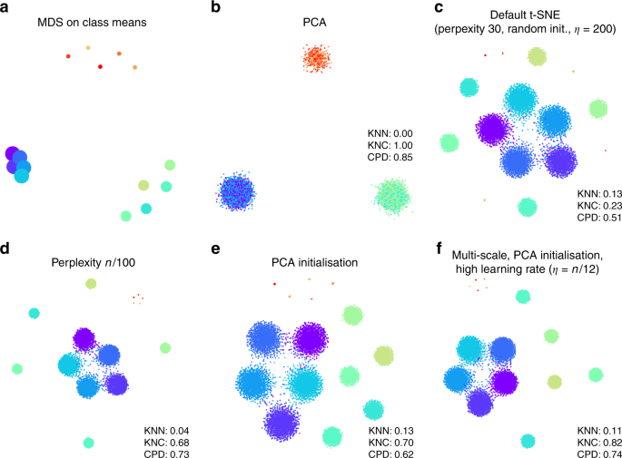
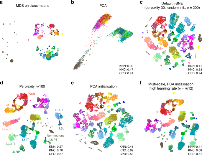
Two classical methods to visualise high-dimensional data are multidimensional scaling (MDS) and principal component analysis (PCA). MDS is difficult to compute with a large number of points (here n = 15,500), but can be easily applied to class means ( \(n=15\) ), clearly showing the three distinct classes (Fig. 1a). PCA can be applied to the whole data set and demonstrates the same large-scale structure of the data (Fig. 1b), but no within-class structure can be seen in the first two PCs. In contrast, t-SNE clearly shows all 15 types, correctly displaying ten of them as fully isolated and five as partially overlapping (Fig. 1c). However, the isolated types end up arbitrarily placed, with their positions mostly depending on the random seed used for initialisation.
In order to quantify numerically the quality, or faithfulness, of a given embedding, we used three different metrics:
Applying these metrics to the PCA and t-SNE embeddings (Fig. 1b, c) shows that t-SNE is much better than PCA in preserving the local structure (KNN 0.13 vs. 0.00) but much worse in preserving the global structure (KNC 0.23 vs. 1.00 and CPD 0.51 vs. 0.85). Our recipe for a more faithful t-SNE visualisation is based on three ideas that have been previously suggested in various contexts: multi-scale similarities 13,14 , PCA initialisation, and increased learning rate 15 .
Fig. 1c used perplexity 30, which is the default value in most t-SNE implementations. Much larger values can yield qualitatively different outcomes. As large perplexity yields longer-ranging attractive forces during t-SNE optimisation, the visualisation loses some fine detail but pulls larger structures together. As a simple rule of thumb, we take 1% of the sample size as a large perplexity for any given data set; this corresponds to perplexity 155 for our simulated data and results in five small clusters belonging to the same class attracted together (Fig. 1d). Our metrics confirmed that, compared to the standard perplexity value, the local structure (KNN) deteriorates but the global structure (KNC and CPD) improves. A multi-scale approach, using multiple perplexity values at the same time, has been previously suggested to preserve both local and global structure 13,14 . We adopt this approach in our final pipeline and, whenever \(n/100\gg 30\) , combine perplexity 30 with the large perplexity \(n/100\) (see below; separate evaluation not shown here).
Another approach to preserve global structure is to use an informative initialisation, e.g. the first two PCs (after appropriate scaling, see Methods). This injects the global structure into the t-SNE embedding which is then preserved during the course of t-SNE optimisation while the algorithm optimises the fine structure (Fig. 1e). Indeed, KNN did not depend on initialisation, but both KNC and CPD markedly improved when using PCA initialisation. PCA initialisation is also convenient because it makes the t-SNE outcome reproducible and not dependent on a random seed.
The third ingredient in our t-SNE protocol is to increase the learning rate. The default learning rate in most t-SNE implementations is \(\eta =200\) which is not enough for large data sets and can lead to poor convergence and/or convergence to a suboptimal local minimum 15 . A recent Python library for scRNA-seq analysis, scanpy , increased the default learning rate to 1000 23 , whereas ref. 15 suggested to use \(\eta =n/12\) . We adopt the latter suggestion and use \(\eta =n/12\) whenever it is above 200. This does not have a major influence on our synthetic data set (because its sample size is not large enough for this to matter), but will be important later on.
Putting all three modifications together, we obtain the visualisation shown in Fig. 1f. The quantitative evaluation confirmed that in terms of the mesoscopic/macroscopic structure, our suggested pipeline strongly outperformed the default t-SNE and was better than large perplexity or PCA initialisation on their own. At the same time, in terms of the miscroscopic structure, it achieved a compromise between the small and the large perplexities.
To demonstrate these ideas on a real-life data set, we chose to focus on the data set from Tasic et al. 3 . It encompasses 23,822 cells from adult mouse cortex, split by the authors into 133 clusters with strong hierarchical organisation. Here and below we used a standard preprocessing pipeline consisting of sequencing depth normalisation, feature selection, log-transformation, and reducing the dimensionality to 50 PCs (see Methods).
In the Tasic et al. data, three well-separated groups of clusters are apparent in the MDS (Fig. 2a) and PCA (Fig. 2b) plots, corresponding to excitatory neurons (cold colours), inhibitory neurons (warm colours), and non-neural cells such as astrocytes or microglia (grey/brown colours). Performing PCA on these three data subsets separately (Supplementary Fig. 1) reveals further structure inside each of them: e.g. inhibitory neurons are well separated into two groups, Pvalb/SSt-expressing (red/yellow) and Vip/Lamp5-expressing (purple/salmon), as can also be seen in Fig. 2a. This demonstrates the hierarchical organisation of the data.
This global structure is missing from a standard t-SNE visualisation (Fig. 2c): excitatory neurons, inhibitory neurons, and non-neural cells are all split into multiple islands that are shuffled among each other. For example, the group of purple clusters (Vip interneurons) is separated from a group of salmon clusters (a closely related group of Lamp5 interneurons) by some excitatory clusters, misrepresenting the hierarchy of cell types. This outcome is not a strawman: the original paper 3 features a t-SNE figure qualitatively very similar to our visualisation. Perplexity values in the common range (e.g. 20, 50, 80) yield similar results, confirming that t-SNE is not very sensitive to the exact value of perplexity.
In contrast, setting perplexity to 1% of the sample size, in this case to 238, pulls together large groups of related types, improving the global structure (KNC and CPD increase), at the expense of losing some of the fine structure (KNN decreases, Fig. 2d). PCA initialisation with default perplexity also improves the global structure (KNC and CPD increase, compared to the default t-SNE, Fig. 2e). Finally, our suggested pipeline with multi-scale similarities (perplexity combination of 30 and \(n/100=238\) ), PCA initialisation, and learning rate \(n/12 \approx 2000\) yields an embedding with high values of all three metrics (Fig. 2f). Compared to the default parameters, these settings slowed down FIt-SNE from \(\sim\) 30 s to \(\sim\) 2 m, which we still find to be an acceptable runtime.
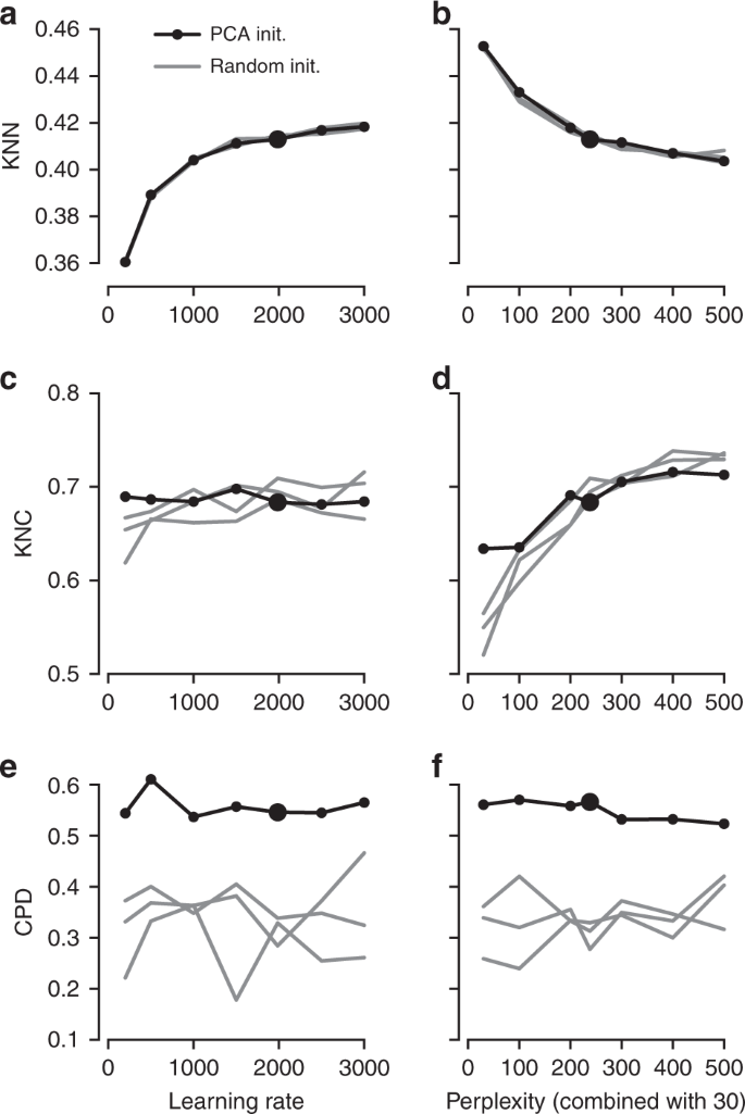
It is instructive to study systematically how the choice of parameters influences the embedding quality (Fig. 3). We found that the learning rate only influences KNN: the higher the learning rate, the better preserved is the local structure, until is saturates at around \(n/10\) (Fig. 3a), in agreement with the results of ref. 15 . The other two metrics, KNC and CPD, are not affected by the learning rate (Fig. 3c, e). The perplexity controls the trade-off between KNN and KNC: the higher the perplexity combined with 30, the worse is the microscropic structure (Fig. 3b) but the better is the mesoscopic structure (Fig. 3d). Our choice of \(n/100\) provides a reasonable compromise. Finally, the PCA initialisation strongly improves the macroscopic structure as measured by the CPD (Fig. 3e, f), while the other two parameters have little influence on it.
To demonstrate that our approach is equally well applicable to UMI-based transcriptomic data, we considered three further data sets. First, we analysed a n = 44,808 mouse retina data set from ref. 24 . Our t-SNE result preserved much of the global geometry (Fig. 4a): e.g. multiple amacrine cell clusters (green), bipolar cell clusters (blue), and non-neural clusters (magenta) were placed close together. The t-SNE analysis performed by the authors in the original publication relied on downsampling and had a worse representation of the cluster hierarchy.
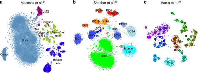
Second, we analysed a n = 27,499 data set from ref. 25 that sequenced cells from mouse retina targeting bipolar neurons. Here again, our t-SNE result (Fig. 4b) is consistent with the global structure of the data: for example, OFF bipolar cells (types 1–4, warm colours) and ON bipolar cells (types 5–9, cold colours) are located close to each other, and four subtypes of type 5 are also close together. This was not true for the t-SNE shown in the original publication. This data set shows one limitation of our method: the data contain several very distinct but very rare clusters and those appear in the middle of the embedding, instead of being placed far out on the periphery (see Discussion).
Finally, we analysed a \(n=3663\) data set of hippocampal interneurons from ref. 26 . The original publication introduced a novel clustering and feature selection method based on the negative binomial distribution, and used a modified negative binomial t-SNE procedure. Our t-SNE visualisation (Fig. 4c) did not use any of that but nevertheless led to an embedding very similar to the one shown in the original paper. Note that for data sets of this size, our method uses perplexity and learning rate that are close to the default ones.
A common task in single-cell transcriptomics is to match a given cell to an existing reference data set. For example, introducing a protocol called Patch-seq, ref. 27 performed patch-clamp electrophysiological recordings followed by RNA sequencing of inhibitory cells in layer 1 of mouse visual cortex. Given the existence of the much larger Tasic et al. data set described above, it is natural to ask where on the Fig. 2f, taken as a reference atlas, these Patch-seq cells should be positioned.
It is often claimed that t-SNE does not allow out-of-sample mapping, i.e. no new points can be put on a t-SNE atlas after it is constructed. What this means is that t-SNE is a nonparametric method that does not construct any mapping \(<\mathrm
An important caveat is that this method assumes that for each new cell there are cells of the same type in the reference data set. Cells that do not have a good match in the reference data can end up positioned in a misleading way. However, this assumption is justified whenever cells are mapped to a comprehensive reference atlas covering the same tissue, as in the example case shown here.
In a more sophisticated approach 24,29,30 , each new cell is initially positioned as outlined above but then its position is optimised using the t-SNE loss function: the cell is attracted to its nearest neighbours in the reference set, with the effective number of nearest neighbours determined by the perplexity. We found that the simpler procedure without this additional optimisation step worked well for our data; the additional optimisation usually has only a minor effect 30 .
We can demonstrate the consistency of our method by a procedure similar to a leave-one-out cross-validation. We repeatedly removed one random Tasic et al. cell from the Vip/Lamp5 clusters, and positioned it back on the same reference t-SNE atlas (excluding the same cell from the \(k=10\) nearest neighbours). Across 100 repetitions, the average distance between the original cell location and the test positioning was \(3.2\pm 2.4\) (mean \(\pm\) SD; see Fig. 5b for a scale bar), and most test cells stayed within their clusters.
Positioning uncertainty can be estimated using bootstrapping across genes (inspired by ref. 3 ). For each of the Patch-seq cells, we repeatedly selected a bootstrapped sample from the set of highly variable genes and repeated the positioning procedure (100 times). This yielded a set of bootstrapped mapping locations; the larger the variability in this set, the larger the uncertainty. To visualise the uncertainty, we show a convex hull covering 95% of the bootstrap repetitions (Fig. 5c), which can be interpreted as a 2D confidence interval. A large polygon means high uncertainty; a small polygon means high precision. For some cells the polygons are so small that they are barely visible in Fig. 5c. For some other cells the polygons are larger and sometimes spread across the border of two adjacent clusters. This suggests that the cluster assignments for these cells are not certain.
Tasic et al. 3 is a follow-up to Tasic et al. 31 where \(n=1679\) cells from mouse visual cortex were sequenced with an earlier sequencing protocol. If one excludes from the new data set all clusters that have cells mostly from outside of the visual cortex, then the remaining data set has \(n=19,\!366\) cells. How similar is the cluster structure of this newer and larger data set compared to the older and smaller one? One way to approach this question is through aligned t-SNE visualisations.
To obtain aligned t-SNE visualisations, we first performed t-SNE of the older data set 31 using PCA initialisation and perplexity 50 (Fig. 6a). We then positioned cells of the newer data set 3 on this reference using the procedure described above and used the resulting layout as initialisation for t-SNE (with learning rate \(n/12\) and perplexity combination of 30 and \(n/100\) , as elsewhere). The resulting t-SNE embedding is aligned to the previous one (Fig. 6b).
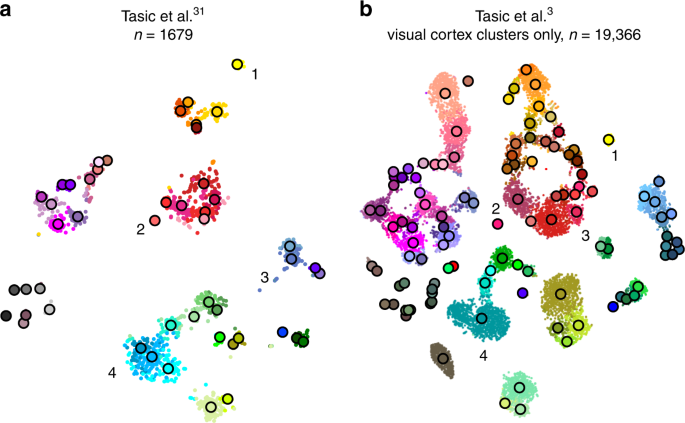
Several observations are highlighted in Fig. 6. (1) and (2) are examples of well-isolated clusters in the 2016 data that remained well-isolated in the 2018 data (Sst Chodl and Pvalb Vipr2; here and below we use the 2018 nomenclature). (3) is an example of a small group of cells that was not assigned to a separate cluster back in 2016, became separate on the basis of the 2018 data, but in retrospect appears well-isolated already in the 2016 t-SNE plot (two L5 LP VISp Trhr clusters). Finally, (4) shows an example of several clusters in the 2016 data merging together into one cluster based on the 2018 data (L4 IT VISp Rspo1). These observations are in good correspondence with the conclusions of ref. 3 , but we find that t-SNE adds a valuable perspective and allows for an intuitive comparison.
Large data sets with \(n\gg 100,000\) present several additional challenges to those already discussed above. First, vanilla t-SNE 9 is slow for \(n\gg 1000\) and computationally unfeasible for \(n\gg 10,\!000\) (see Methods). A widely used approximation called Barnes-Hut t-SNE 32 in turn becomes very slow for \(n\gg 100,\!000\) . For larger data sets a faster approximation scheme is needed. This challenge was effectively solved by ref. 16 who developed a novel t-SNE approximation called FIt-SNE, based on an interpolation scheme accelerated by the fast Fourier transform. Using FIt-SNE, we were able to process a data set with 1 million points and 50 dimensions (perplexity 30) in 29 min on a computer with four 3.4 GHz double-threaded cores, and in 11 min on a server with twenty 2.2 GHz double-threaded cores.
Second, for \(n\gg 100,\!000\) , t-SNE with default optimisation parameters tends to produce poorly converged solutions and embeddings with continuous clusters fragmented into several parts. Various groups 16,23 have noticed that these problems can be alleviated by increasing the number of iterations, the length or strength of the early exaggeration (see Methods), or the learning rate. Ref. 15 demonstrated in a thorough investigation that dramatically increasing the learning rate from the default value \(\eta =200\) to \(\eta =n/12\) (where 12 is the early exaggeration coefficient 33 ) prevents cluster fragmentation during the early exaggeration phase and yields a well-converged solution within the default 1000 iterations.
Third, for \(n\gg 100,\!000\) , t-SNE embeddings tend to become very crowded, with little white space even between well-separated clusters 18 . The exact mathematical reason for this is not fully understood, but the intuition is that the default perplexity becomes too small compared to the sample size, repulsive forces begin to dominate, and clusters blow up and coalesce like adjacent soap bubbles. While so far there is no principled solution for this in the t-SNE framework, a very practical trick suggested by ref. 34 is to increase the strength of all attractive forces by a small constant exaggeration factor between 1 and \(\sim\) 10 (see Methods). This counteracts the expansion of the clusters.
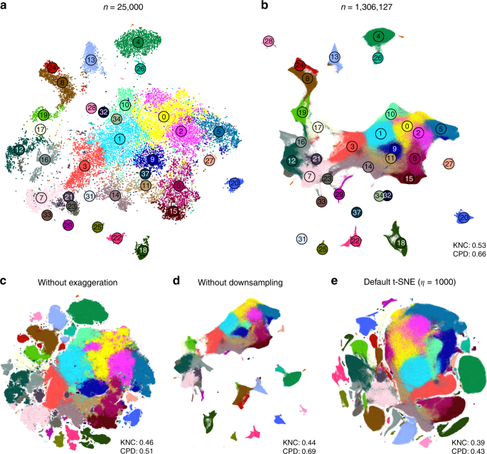
Fourth, our approach to preserve global geometry relies on using large perplexity \(n/100\) and becomes computationally unfeasible for \(n\gg 100,\!000\) because FIt-SNE runtime grows linearly with perplexity. For such sample sizes, the only practical possibility is to use perplexity values in the standard range 10–100. To address this challenge, we make an assumption that global geometry should be detectable even after strong downsampling of the data set. This suggests the following pipeline: (i) downsample a large data set to some manageable size; (ii) run t-SNE on the subsample using our approach to preserve global geometry; (iii) position all the remaining points on the resulting t-SNE plot using nearest neighbours; (iv) use the result as initialisation to run t-SNE on the whole data set.
We demonstrate these ideas using two currently largest scRNA-seq data sets. The first one is a 10x Genomics data set with \(n=1,\!306,\!127\) cells from mouse embryonic brain. We first created a t-SNE embedding of a randomly selected subset of \(n=25,\!000\) cells (Fig. 7a). As above, we used PCA initialisation, perplexity combination of 30 and \(n/100=250\) , and learning rate \(n/12\) . We then positioned all the remaining cells on this t-SNE embedding using their nearest neighbours (here we used Euclidean distance in the PCA space, and \(k=10\) as above; this took \(\sim\) 10 min). Finally, we used the result as initialisation to run t-SNE on all points using perplexity 30, exaggeration coefficient 4, and learning rate \(n/12\) (Fig. 7b).
To validate this procedure, we identified meaningful biological structures in the embedding using developmental marker genes 35,36,37 . The left part of the main continent is composed of radial glial cells expressing Aldoc and Slc1a3 (Fig. 8a). The neighbouring areas consist of neural progenitors (neuroblasts) expressing Eomes, previously known as Tbr2 (Fig. 8b). The right part of the main continent consists of mature excitatory neurons expressing pan-neuronal markers such as Stmn2 and Tubb3 (Fig. 8c) but not expressing inhibitory neuron markers Gad1 or Gad2 (Fig. 8d), whereas the upper part of the embedding is occupied by several inhibitory neuron clusters (Fig. 8d). This confirms that our t-SNE embedding shows meaningful topology and is able to capture the developmental trajectories: from radial glia, to excitatory/inhibitory neural progenitors, to excitatory/inhibitory mature neurons.
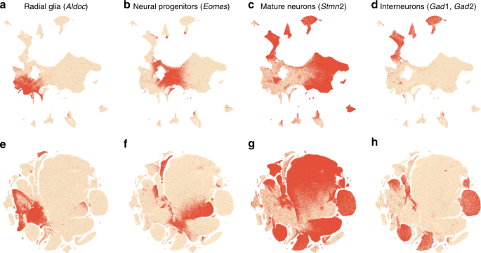
We illustrate the importance of the components of our pipeline by a series of control experiments. Omitting exaggeration yielded over-expanded clusters and less discernible global structure (Fig. 7c). Without downsampling, the global geometry was preserved worse (Fig. 7d): e.g. most of the interneuron clusters are in the lower part of the figure, but clusters 17 and 19 (developing interneurons) are located in the upper part. Finally, the default t-SNE with random initialisation and no exaggeration (but learning rate set to \(\eta =1000\) ) yielded a poor embedding that fragmented some of the clusters and misrepresented global geometry (Fig. 7e). Indeed, overlaying the same marker genes showed that developmental trajectories were not preserved and related groups of cells, e.g. interneurons, were dispersed across the embedding (Fig. 8e–h). Again, this is not a strawman: this embedding is qualitatively similar to the ones shown in the literature 23,38 .
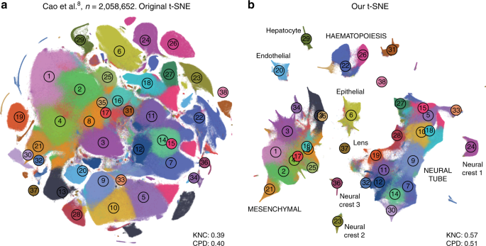
In addition, we analysed a data set encompassing \(n=2,\!058,652\) cells from mouse embryo at several developmental stages 8 . The original publication showed a t-SNE embedding that we reproduced in Fig. 9a. Whereas it showed a lot of structure, it visibly suffered from all the problems mentioned above: some clusters were fragmented into parts (e.g. clusters 13 and 15), there was little separation between distinct cell types, and global structure was grossly misrepresented. The authors annotated all clusters and split them into ten biologically meaningful developmental trajectories; these trajectories were intermingled in their embedding. In contrast, our t-SNE embedding (Fig. 9b) neatly separated all ten developmental trajectories and arranged clusters within major trajectories in a meaningful developmental order: e.g. there was a continuous progression from radial glia (cluster 7), to neural progenitors (9), to postmitotic premature neurons (10), to mature excitatory (5) and inhibitory (15) neurons.
A promising dimensionality reduction method called UMAP 10 has recently attracted considerable attention in the transcriptomics community 11 . Technically, UMAP is very similar to an earlier method called largeVis 39 , but ref. 10 provided a mathematical foundation and a convenient Python implementation. LargeVis and UMAP use the same attractive forces as t-SNE does, but change the nature of the repulsive forces and use a different, sampling-based approach to optimisation. UMAP has been claimed to be faster than t-SNE and to outperform it in terms of preserving the global structure of the data 10,11 .
While UMAP is indeed much faster than Barnes-Hut t-SNE, FIt-SNE 16 is at least as fast as UMAP. We found FIt-SNE 1.1 with default settings to be \(\sim\) 4 times faster than UMAP 0.3 with default settings when analysing the 10x Genomics (14 m vs. 56 m) and the Cao et al. (31 m vs. 126 m) data sets on a server with twenty 2.2 GHz double-threaded cores (for this experiment, the input dimensionality was 50 and the output dimensionality was 2; UMAP may be more competitive in other settings). That said, the exact runtime will depend on the details of implementation, and both methods may be further accelerated in future releases, or by using GPU parallelisation 40 .
To compare UMAP with our t-SNE approach in terms of preservation of global structure, we first ran UMAP on the synthetic and on the Tasic et al. 3 data sets (Supplementary Fig. 2). We used the default UMAP parameters, and also modified the two key parameters (number of neighbours and tightness of the embedding) to produce a more t-SNE-like embedding. In both cases and for both data sets, all three metrics (KNN, KNC, and CPD) were considerably lower than with our t-SNE approach. Notably, we observed that in some cases the global structure of UMAP embeddings strongly depended on the random seed. Next, we applied UMAP with default parameters to the 10x Genomics and the Cao et al. data sets. Here UMAP embeddings were qualitatively similar to our t-SNE embeddings, but arguably misrepresented some aspects of the global topology (Supplementary Fig. 3).
An in-depth comparison of t-SNE and UMAP is beyond the scope of our paper, but this analysis suggests that previous claims that UMAP vastly outperforms t-SNE 11 might have been partially due to t-SNE being applied in a suboptimal way. Our analysis also indicates that UMAP does not necessarily solve t-SNE’s problems out of the box and might require as many careful parameter and/or initialisation choices as t-SNE does. Many recommendations for running t-SNE that we made in this manuscript can likely be adapted for UMAP.
The fact that t-SNE does not always preserve global structure is one of its well-known limitations 12 . Indeed, the algorithm, by construction, only cares about preserving local neighbourhoods. We showed that using informative initialisation (such as PCA initialisation, or downsampling-based initialisation) can substantially improve the global structure of the final embedding because it survives through the optimisation process. Importantly, a custom initialisation does not interfere with t-SNE optimisation and does not yield a worse solution compared to a random initiliasation used by default (Fig. 3a, b). A possible concern is that a custom initialisation might bias the resulting embedding by injecting some artefact global structure. However, if anything can be seen as injecting artefactual structure, it is rather the random initialisation: the global arrangement of clusters in a standard t-SNE embedding often strongly depends on the random seed.
We also showed that using large perplexity values ( \(\sim\) 1% of the sample size)—substantially larger than the commonly used ones—can be useful in the scRNA-seq context. Our experiments suggest that whereas PCA initialisation helps preserving the macroscropic structure, large perplexity (either on its own or as part of a perplexity combination) helps preserving the mesoscopic structure (Fig. 3d, f).
It has recently been claimed that UMAP preserves the global geometry better than t-SNE 11 . However, UMAP operates on the \(k\) -nearest neighbour graph, exactly as t-SNE does, and is therefore not designed to preserve large distances any more than t-SNE. To give a specific example, ref. 8 , performed both t-SNE and UMAP and observed that “unlike t-SNE, UMAP places related cell types near one another”. We demonstrated that this is largely because t-SNE parameters were not set appropriately. Simply using high learning rate \(n/12\) places related cell types near one another as well as UMAP does, and additionally using exaggeration factor \(4\) separates clusters into more compact groups, similar to UMAP.
T-SNE is often perceived as having only one free parameter to tune, perplexity. Under the hood, however, there are also various optimisation parameters (such as the learning rate, the number of iterations, early exaggeration factor, etc.) and we showed above that they can have a dramatic effect on the quality of the visualisation. Here we have argued that exaggeration can be used as another useful parameter when embedding large data sets. In addition, while the low-dimensional similarity kernel in t-SNE has traditionally been fixed as the t-distribution with \(\nu =1\) degree of freedom, we showed in a parallel work that modifying \(\nu\) can uncover additional fine structure in the data 41 .
One may worry that this gives a researcher too many knobs to turn. However, here we gave clear guidelines on how to set these parameters for effective visualisations. As argued above and in ref. 15 , setting the learning rate to \(n/12\) ensures good convergence and automatically takes care of the optimisation issues. Perplexity should be left at the default value 30 for very large data sets, but can be combined with \(n/100\) for smaller data sets. Exaggeration can be increased to \(\sim\) 4 for very large data sets, but is not needed for smaller data sets.
In comparison, UMAP has two main adjustable parameters (and many further optimisation parameters): n_neighbors , corresponding to perplexity, and min_dist , controlling how tight the clusters become. The latter parameter sets the shape of the low-dimensional similarity kernel 10 and is therefore analogous to \(\nu\) mentioned above. Our experiments with UMAP suggest that its repulsive forces roughly correspond to t-SNE with exaggeration \(\sim\) 4 (Supplementary Figs. 2, 3). Whether this is desirable, depends on the application. With t-SNE, one can choose to switch exaggeration off and e.g. use the embedding shown in Fig. 7c instead of Fig. 7b.
Several variants of t-SNE have been recently proposed in the literature. One important example is parametric t-SNE, where a neural network is used to create a mapping \(<\mathrm
Another important development is hierarchical t-SNE, or HSNE 45 . The key idea is to use random walks on the \(k\) -nearest neighbours graph of the data to find a smaller set of landmarks, which are points that can serve as representatives of the surrounding points. In the next round, the \(k\) -nearest neighbours graph on the level of landmarks is constructed. This operation can reduce the size of the data set by an order of magnitude, and can be repeated until the data set becomes small enough to be analysed with t-SNE. Each level of the landmarks hierarchy can be explored separately. Ref. 18 successfully applied this method to mass cytometry data sets with up to 15 million cells. However, HSNE does not allow to embed all \(n\) points in a way that would preserve the geometry on the level of landmarks.
Our approach to preserving global geometry of the data is based on using PCA initialisation and large perplexity values. It can fail if some aspects of the global geometry are not adequately captured in the first two PCs or by the similarities computed using a large perplexity. This may happen when the data set contains very isolated but rare cell types. Indeed, a small isolated cluster might not appear isolated in the first two PCs because it would not have enough cells to contribute much to the explained variance. At the same time, large perplexity will make the points in that cluster be attracted to some arbitrary, unrelated, clusters. As a result, a small cluster can get sucked into the middle of the embedding even if it is initialised on the periphery.
This is what happened in the Shekhar et al. data set (Fig. 4b): cone and rod photoreceptor (yellow) and amacrine cell (cyan) clusters ended up in the middle of the embedding despite being very different from all the bipolar cell clusters. This can be seen in the MDS embedding of the cluster means which is unaffected by the relative abundances of the clusters; thus, when t-SNE is done together with clustering, we recommend to supplement a t-SNE visualisation with a MDS visualisation of cluster means (as in Fig. 2a). Alternatively, one could use PAGA 46 , a recent method specifically designed to visualise the relationships between clusters in scRNA-seq data.
This example highlights that our approach is not a final solution to preserving the global structure of the data. A principled approach would incorporate some terms ensuring adequate global geometry directly into the loss function, while making sure that the resulting algorithm is scalable to millions of points. We consider it an important direction for future work. In the meantime, we believe that our recommendations will strongly improve t-SNE visualisations used in the current single-cell transcriptomic studies, and may be useful in other application domains as well.
The t-SNE algorithm 9 is based on the SNE framework 47 . SNE introduced a notion of directional similarity of point \(j\) to point \(i\) ,